Pointing Matrix
%matplotlib inline
%config InlineBackend.figure_format = "retina"
import matplotlib.pyplot as plt
import numpy as np
import seaborn as sns
sns.set()
plt.rcParams['figure.figsize'] = (10.0, 6.0)
import sympy as sym
from sympy.vector import CoordSys3D

sym.init_printing()
Background
The "Pointing Matrix" in TOAST is represented by two types of operations. The first is the mapping from geometric detector quaternion pointing to a pixelized representation of the sky. The second is the model of the detector response to incoming polarized light. This model can be expressed as the application of Mueller matrices representing optical elements in the system. The incoming light can be expressed as a vector of Stokes parameters I, Q, U, and V.
The Stokes parameters are defined with respect to the local meridian at the detector line of sight. In the TOAST formalism, the detector frame has the Z axis pointing along the detector line of sight and the X axis aligned with the direction of maximum polarization response. For this exercise, we will use the COSMO convention for the Stokes parameters, since it conveniently also has the Z axis along the line of sight. The final result is easy to swap between COSMO / IAU simply by changing the sign of the U Stokes parameter. In some scenarios, it can be convenient to look at the various angles from the perspective of the instrument "looking out" at the sky (with the detector Z axis going "into the page"). In other cases it makes more sense to visualize the situation "looking in" from the sky. The figures below clearly label which case is being displayed.
Definitions
We will use $alpha$ to represent the angle of right-handed rotation from the meridian to the detector polarization orientation (the detector frame X axis) about the line of sight (detector Z axis). We use $omega$ to represent the right-handed angle of rotation, about the line of sight, from the meridian to a direction parallel to the HWP fast axis. The cross-polar leakage of the linearly polarized detector is $epsilon$. To visually simplify things, we define the polarization coefficient:
$$ C = \frac{1 - \epsilon}{1 + \epsilon} $$
And note that there is a factor of $1/2$ that can be included in an overall calibration factor in the resulting measured output power.
alpha = sym.Symbol(r"\alpha")
omega = sym.Symbol(r"\omega")
epsilon = sym.Symbol(r"\epsilon")
C = sym.Symbol("C")
alpha, omega, epsilon, C
Mueller Matrix Representation
Assume we have an input Stokes vector:
$$ \vec{S}_{in} = \left[ \begin{array}{c} I_{in}\\ Q_{in}\\ U_{in}\\ V_{in} \end{array} \right] $$
In the case of no HWP and just a partial linear polarizer followed by a total power measurement, the resulting measured power is:
$$ P_{out} = \mathbf{T}_{power} \cdot \mathbf{M}_{det} \;\vec{S}_{in} $$
Where the total power measurement $\mathbf{T}$ is simply the sum of the top row of the final Mueller matrix. If we introduce a rotating HWP followed by the fixed linear polarizer and then a total power measurement we get:
$$ P_{out} = \mathbf{T}_{power} \cdot \mathbf{M}_{det} \cdot \mathbf{M}_{HWP}(t) \;\vec{S}_{in} $$
The detector and HWP Mueller matrices include a rotational coordinate transform:
$$ \mathbf{M}_{HWP} = \mathbf{R}_{HWP}^{-1}\; \mathbf{M}_{Fixed\ HWP}\; \mathbf{R}_{HWP} $$
Where the rotation matrix transforms from the measurement frame to the local coordinates of the HWP. Similarly the detector Mueller matrix is an (imperfect) linear polarizer with some rotation from the measurement frame:
$$ \mathbf{M}_{det} = \mathbf{R}_{det}^{-1}\; \mathbf{M}_{Linear\ Pol}\; \mathbf{R}_{det} $$
HWP Matrix
The ideal, local HWP has Mueller matrix of:
# Ideal HWP in local frame:
Lhwp = sym.Matrix([
    [1, 0, 0, 0],
    [0, 1, 0, 0],
    [0, 0, -1, 0],
    [0, 0, 0, -1],
])
Lhwp
and the rotation matrix from the coordinate frame to the local frame is:
Rhwp = sym.Matrix([
    [1, 0, 0, 0],
    [0, sym.cos(2 * omega), -sym.sin(2 * omega), 0],
    [0, sym.sin(2 * omega), sym.cos(2 * omega), 0],
    [0, 0, 0, 1],
])
Rhwp
For simplifying the algebra below, we use $b = 2\omega$. The inverse coordinate transform is a result of swapping $\omega$ for $-\omega$.
b = sym.Symbol(r"b")

Rhwp = sym.Matrix([
    [1, 0, 0, 0],
    [0, sym.cos(b), -sym.sin(b), 0],
    [0, sym.sin(b), sym.cos(b), 0],
    [0, 0, 0, 1],
])
Rhwp
Rhwpinv = sym.Matrix([
    [1, 0, 0, 0],
    [0, sym.cos(b), sym.sin(b), 0],
    [0, -sym.sin(b), sym.cos(b), 0],
    [0, 0, 0, 1],
])
Rhwpinv
And then the final HWP Mueller matrix becomes:
Mhwp = sym.simplify(Rhwpinv * Lhwp * Rhwp)
Mhwp
Linearly Polarized Detector
A (partial) linear polarizer has the local Mueller matrix:
Ldet = sym.Matrix([
    [1, C, 0, 0],
    [C, 1, 0, 0],
    [0, 0, 0, 0],
    [0, 0, 0, 0],
])
Ldet
The Mueller matrix which rotates a Stokes vector in a right-handed counter-clockwise sense from the coordinate frame to the local frame is again given by:
Rdet = sym.Matrix([
    [1, 0, 0, 0],
    [0, sym.cos(2 * alpha), -sym.sin(2 * alpha), 0],
    [0, sym.sin(2 * alpha), sym.cos(2 * alpha), 0],
    [0, 0, 0, 1],
])
Rdet
For simplifying the algebra below, we use $a = 2\alpha$.
a = sym.Symbol(r"a")
Rdet = sym.Matrix([
    [1, 0, 0, 0],
    [0, sym.cos(a), -sym.sin(a), 0],
    [0, sym.sin(a), sym.cos(a), 0],
    [0, 0, 0, 1],
])
Rdet
The inverse transform can be obtained by evaluating this at $-\alpha$
Rdetinv = sym.Matrix([
    [1, 0, 0, 0],
    [0, sym.cos(a), sym.sin(a), 0],
    [0, -sym.sin(a), sym.cos(a), 0],
    [0, 0, 0, 1],
])
Rdetinv
The final detector Mueller matrix in the measurement frame is then:
Mdet = sym.simplify(Rdetinv * Ldet * Rdet)
Mdet
Final Expression - Without HWP
The optical response without a HWP is just the linear polarized detector result above. The output Stokes weights are:
s_I = Mdet[0, 0]
s_I
s_Q = Mdet[0, 1]
s_Q
s_U = Mdet[0, 2]
s_U
So the final measured power is:
$$ P_{out} = \frac{1}{2} \left[ I_{in} + \frac{1 - \epsilon}{1 + \epsilon} \left[ Q_{in} \cos \left( 2 \alpha \right) + U_{in} \sin \left( 2 \alpha \right) \right] \right]\qquad (COSMO) $$
OR
$$ P_{out} = \frac{1}{2} \left[ I_{in} + \frac{1 - \epsilon}{1 + \epsilon} \left[ Q_{in} \cos \left( 2 \alpha \right) - U_{in} \sin \left( 2 \alpha \right) \right] \right]\qquad (IAU) $$
Consider the trivial case where the focalplane coordinates are aligned with the coordinate axes, so that $\alpha$ is exactly the orientation of the detector in the coordinate frame. For several different $\alpha$ values (in COSMO convention) we have:
$$ \begin{aligned} Q_{weight}(\alpha = 0) = & \;1 \\ U_{weight}(\alpha = 0) = & \;0 \end{aligned} $$
$$ \begin{aligned} Q_{weight}(\alpha = 45) = & \;0 \\ U_{weight}(\alpha = 45) = & \;1 \end{aligned} $$
$$ \begin{aligned} Q_{weight}(\alpha = 90) = & \;-1 \\ U_{weight}(\alpha = 90) = & \;0 \end{aligned} $$
Final Expression - Including HWP
The combined optical response of the HWP and detector matrices are then:
Mopt = sym.simplify(Mdet * Mhwp)
Mopt
And the output Stokes weights are:
s_I = Mopt[0, 0]
s_I
s_Q = Mopt[0, 1]
s_Q
s_U = Mopt[0, 2]
s_U
So the final measured power is:
$$ P_{out} = \frac{1}{2} \left[ I_{in} + \frac{1 - \epsilon}{1 + \epsilon} \left[ Q_{in} \cos \left( 2(\alpha - 2\omega) \right) - U_{in} \sin \left( 2(\alpha - 2\omega) \right) \right] \right]\qquad (COSMO) $$
OR
$$ P_{out} = \frac{1}{2} \left[ I_{in} + \frac{1 - \epsilon}{1 + \epsilon} \left[ Q_{in} \cos \left( 2(\alpha - 2\omega) \right) + U_{in} \sin \left( 2(\alpha - 2\omega) \right) \right] \right]\qquad (IAU) $$
Consider the trivial case where the focalplane coordinates are aligned with the coordinate axes, so that $\alpha$ and $\omega$ are directly the orientations of the detector and HWP in the coordinate frame. In that case, consider a fixed HWP aligned with the meridian ($\omega$ = 0) for several different $\alpha$ values (in COSMO convention):
$$ \begin{aligned} Q_{weight}(\alpha = 0) = & \;1 \\ U_{weight}(\alpha = 0) = & \;0 \end{aligned} $$
$$ \begin{aligned} Q_{weight}(\alpha = 45) = & \;0 \\ U_{weight}(\alpha = 45) = & \;-1 \end{aligned} $$
$$ \begin{aligned} Q_{weight}(\alpha = 90) = & \;-1 \\ U_{weight}(\alpha = 90) = & \;0 \end{aligned} $$
Note the sign flip of the U component at 45 degrees, compared to the case without a HWP present in the optical path.
Detector Response in TOAST
Our starting point is a detector quaternion at each sample that rotates the coordinate frame on the sky to the detector frame, with the Z axis along the line of sight and the X axis along the polarization sensitive direction. In the detector frame, the vector along the meridian is offset by an angle of $-\alpha$. Recall that our detector coordinate frame is offset from the overall focalplane frame. The detector frame is also rotated by an angle ${\gamma}_{D}$. The HWP angle (${\gamma}_{H}(t)$) in the detector frame is time varying and measured from the same reference point:
For the case with no HWP, we just need the angle $\alpha$. If we do have a HWP, then we can use the figure above to express $\omega$ in terms of our known quantities. From this we can see that $\omega = \alpha + {\gamma}_{H}(t) - {\gamma}_{D}$. Substituting this we get (using COSMO convention, which is the default):
$$ P_{out} = \frac{1}{2} \left[ I_{in} + \frac{1 - \epsilon}{1 + \epsilon} \left[ Q_{in} \cos \left( 2 \left( \alpha - 2 \left[ \alpha + {\gamma}_{H}(t) - {\gamma}_{D} \right] \right) \right) - U_{in} \sin \left( 2 \left( \alpha - 2 \left[ \alpha + {\gamma}_{H}(t) - {\gamma}_{D} \right] \right) \right) \right] \right] $$
Expanding:
$$ P_{out} = \frac{1}{2} \left[ I_{in} + \frac{1 - \epsilon}{1 + \epsilon} \left[ Q_{in} \cos \left( 2 \left( \alpha - 2 \alpha - 2 {\gamma}_{H}(t) + 2 {\gamma}_{D} \right) \right) - U_{in} \sin \left( 2 \left( \alpha - 2 \alpha - 2 {\gamma}_{H}(t) + 2 {\gamma}_{D} \right) \right) \right] \right] $$
$$ P_{out} = \frac{1}{2} \left[ I_{in} + \frac{1 - \epsilon}{1 + \epsilon} \left[ Q_{in} \cos \left( 2 \left( - \alpha - 2 {\gamma}_{H}(t) + 2 {\gamma}_{D} \right) \right) - U_{in} \sin \left( 2 \left( - \alpha - 2 {\gamma}_{H}(t) + 2 {\gamma}_{D} \right) \right) \right] \right] $$
$$ P_{out} = \frac{1}{2} \left[ I_{in} + \frac{1 - \epsilon}{1 + \epsilon} \left[ Q_{in} \cos \left( 2 \left[ 2 \left( {\gamma}_{D} - {\gamma}_{H}(t) \right) - \alpha \right] \right) - U_{in} \sin \left( 2 \left[ 2 \left( {\gamma}_{D} - {\gamma}_{H}(t) \right) - \alpha \right] \right) \right] \right] $$
This gives us our total power measurement in terms of a fixed, per-detector offset, the HWP angle in the focalplane frame, and the orientation of the detector frame (the $\alpha$ angle) at each sample.
Example
As a sanity check, consider a scenario where the focalplane X axis is aligned with the coordinate system "South" direction in the figure above. Also choose ${\gamma}_{D}$ to be 45 degrees. In this case, $\alpha == {\gamma}_{D}$ and $2\alpha = 90^{\circ}$.
In the case of no HWP and using COSMO convention, we have:
$$ \begin{aligned} Q_{weight}(45) = & \;\cos \left( 2 \alpha \right) \\ Q_{weight}(45) = & \;0 \end{aligned} $$
$$ \begin{aligned} U_{weight}(45) = & \;\sin \left( 2 \alpha \right) \\ U_{weight}(45) = & \;1 \end{aligned} $$
The Stokes Q weight is zero and the Stokes U weight is +1, which makes sense since the detector is aligned with the positive U axis. In the case of a rotating HWP, our Q weight is:
$$ \begin{aligned} Q_{weight} = & \;\cos \left( 2 \left[ 2 \left( {\gamma}_{D} - {\gamma}_{H}(t) \right) - \alpha \right] \right) \\ & \;\text{(substitute ${\gamma}_{D}=\alpha$)} \\ Q_{weight} = & \;\cos \left( 2 \left[ 2 \alpha - 2 {\gamma}_{H}(t) - \alpha \right] \right) \\ Q_{weight} = & \;\cos \left( 2 \alpha - 4 {\gamma}_{H}(t) \right) \end{aligned} $$
and the U weight is:
$$ \begin{aligned} U_{weight} = & \; - \sin \left( 2 \left[ 2 \left( {\gamma}_{D} - {\gamma}_{H}(t) \right) - \alpha \right] \right) \\ & \;\text{(substitute ${\gamma}_{D}=\alpha$)} \\ U_{weight} = & \; - \sin \left( 2 \left[ 2 \alpha - 2 {\gamma}_{H}(t) - \alpha \right] \right) \\ U_{weight} = & \; - \sin \left( 2 \alpha - 4 {\gamma}_{H}(t) \right) \end{aligned} $$
Consider what happens when the fast axis of the HWP is aligned with the detector orientation (${\gamma}_{H} = \alpha = {\gamma}_{D} = 45^{\circ}$). In that scenario we have:
$$ \begin{aligned} Q_{weight}(45,HWP) = & \;\cos \left( - 2 \alpha \right)\\ Q_{weight}(45,HWP) = & \;0 \end{aligned} $$
$$ \begin{aligned} U_{weight}(45,HWP) = & \; - \sin \left( - 2 \alpha \right)\\ U_{weight}(45,HWP) = & \;1 \end{aligned} $$
Implementation
Given the previous equations, for both the HWP and non-HWP cases we need to use our detector pointing to determine the $\alpha$ angle at each sample. We can use our detector quaternions to rotate the sky coordinate axes to the detector frame. The resulting direction (detector Z axis) and orientation (detector X axis / polarization sensitive direction) vectors are:
$$ \vec{V}_{direction} = \vec{V}_{d} = Q_{det} (\hat{Z}) = V_{dx}\,\hat{i} + V_{dy}\,\hat{j} + V_{dz}\,\hat{k} $$ $$ \vec{V}_{orientation} = \vec{V}_{o} = Q_{det} (\hat{X}) = V_{ox}\,\hat{i} + V_{oy}\,\hat{j} + V_{oz}\,\hat{k} $$
N = CoordSys3D("N")
Vdx = sym.Symbol("Vdx")
Vdy = sym.Symbol("Vdy")
Vdz = sym.Symbol("Vdz")
Vox = sym.Symbol("Vox")
Voy = sym.Symbol("Voy")
Voz = sym.Symbol("Voz")
Vd = Vdx * N.i + Vdy * N.j + Vdz * N.k
Vd
Vo = Vox * N.i + Voy * N.j + Voz * N.k
Vo
Given these, we can construct the vector orthogonal to the detector line of sight ($\vec{V}_{d}$) which is aligned with the local meridian:
$$ \vec{V}_{meridian} = \vec{V}_{m} = V_{dz}\cos \left( {\tan}^{-1} \left( \frac{V_{dy}}{V_{dx}} \right) \right)\;\hat{i} + V_{dz}\sin \left( {\tan}^{-1} \left( \frac{V_{dy}}{V_{dx}} \right) \right)\;\hat{j} - \sqrt{1 - V_{dz}^2}\;\hat{k} $$
Vmx = sym.Symbol("Vmx")
Vmy = sym.Symbol("Vmy")
Vmz = sym.Symbol("Vmz")
Vm = Vmx * N.i + Vmy * N.j + Vmz * N.k
Vm
This vector is co-planar with the detector X / Y coordinate axes. The rotation angle from the meridian vector to the detector X axis ($\vec{V}_{o}$) is the $\alpha$ angle above, and is given by (using the fact that $\vec{V}_{d}$ is the normal to the plane):
$$ \alpha = {\tan}^{-1} \left( \frac{ \left( \vec{V}_{m} \times \vec{V}_{o} \right) \cdot \vec{V}_{d}}{\vec{V}_{m} \cdot \vec{V}_{0}} \right) $$
Which in terms of components is:
sym.atan2((Vm.cross(Vo)).dot(Vd), Vm.dot(Vo))
Pulling out the minus sign and formatting nicely we get:
$$ \alpha = {\tan}^{-1} \left( \frac{ V_{dx} (V_{my} V_{oz} - V_{mz} V_{oy}) - V_{dy} (V_{mx} V_{oz} - V_{mz} V_{ox}) + V_{dz} (V_{mx} V_{oy} - V_{my} V_{ox}) }{ V_{mx} V_{ox} + V_{my} V_{oy} + V_{mz} V_{oz} } \right) $$
So computing the Stokes weights at each sample involves appling the detector quaternion to two vectors, a few trig functions to get the components of $\vec{V}_{m}$, and then the calculation of the $\alpha$ angle.
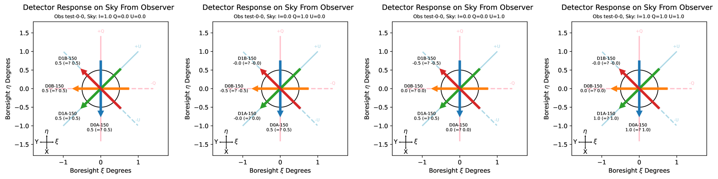
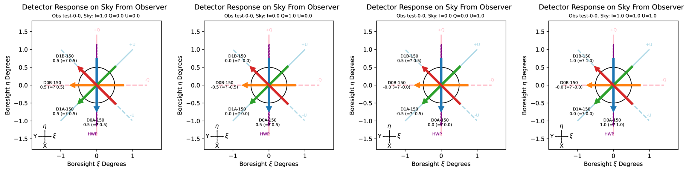
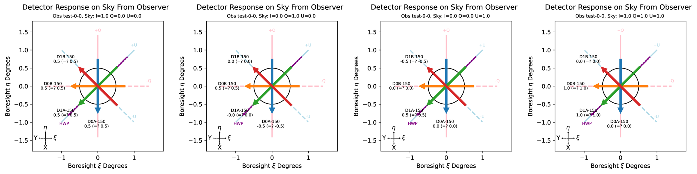
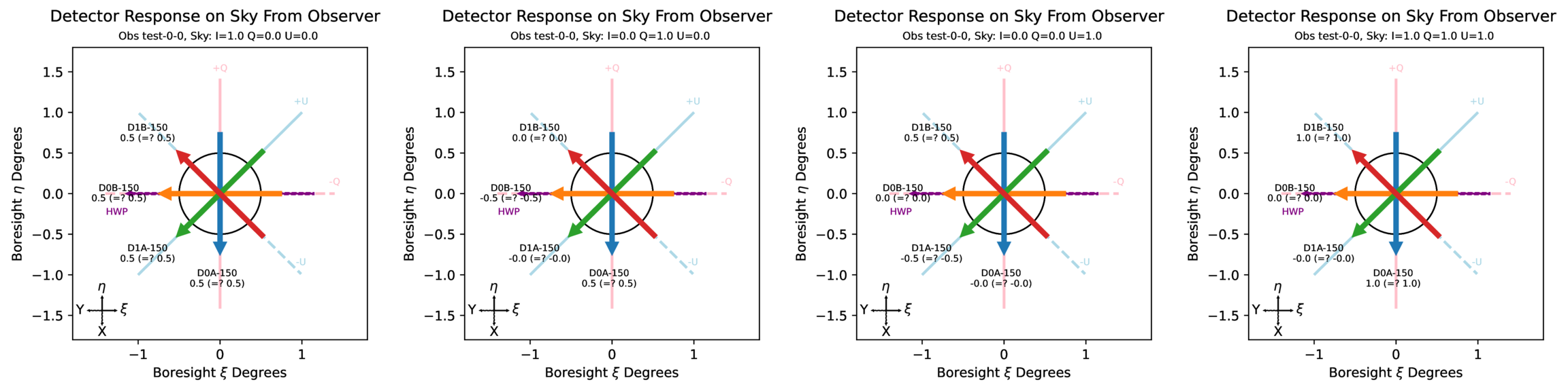
Stokes Weights Unit Tests
The following plots are generated by the unit tests for different cases of input Stokes parameters and HWP state. For each case in the following plots:
The input fake sky has constant I/Q/U values at each pixel, and those are given in the plot subtitle.
The plot is "looking out" from the telescope and the COSMO convention Q/U axes are drawn from this perspective.
The focalplane frame X axis is parallel to the local coordinate system meridian and pointed "South". In other words, the detector gamma angle is exactly equal to the "alpha" angle from the local meridian.
There are 4 detectors at the boresight, and their actual and expected values are given (which should be the same). I am using a calibration factor of $C = 0.5$, so the total response is $0.5[I + q_{weight} * Q + u_{weight} * U]$. The q/u weights are defined in this document above and in the code for the cases with / without a HWP. The cross polar response is set to zero in this test.
Each row represents a different HWP state (including no HWP at all). Each column represents different input map values of $I = 1$, $Q = 1$, $U = 1$, and $I = Q = U = 1$